Setting up and testing hypotheses is an essential part of statistical inference. In order to formulate such a test, usually some theory has been put forward, either because it is believed to be true or because it is to be used as a basis for argument, but has not been proved, for example, claiming that a new drug is better than the current drug for treatment of the same symptoms.

In each problem considered, the question of interest is simplified into two competing claims / hypotheses between which we have a choice; the null hypothesis, denoted H 0. against the alternative hypothesis, denoted H 1. These two competing claims / hypotheses are not however treated on an equal basis: special consideration is given to the null hypothesis.

We have two common situations:

1. The experiment has been carried out in an attempt to disprove or reject a particular hypothesis, the null hypothesis, thus we give that one priority so it cannot be rejected unless the evidence against it is sufficiently strong. For example, H 0. there is no difference in taste between coke and diet coke against H 1. there is a difference.
2. If one of the two hypotheses is ‘simpler’ we give it priority so that a more ‘complicated’ theory is not adopted unless there is sufficient evidence against the simpler one. For example, it is ‘simpler’ to claim that there is no difference in flavour between coke and diet coke than it is to say that there is a difference.

The hypotheses are often statements about population parameters like expected value and variance; for example H 0 might be that the expected value of the height of ten year old boys in the Scottish population is not different from that of ten year old girls. A hypothesis might also be a statement about the distributional form of a characteristic of interest, for example that the height of ten year old boys is normally distributed within the Scottish population.

The outcome of a hypothesis test test is “Reject H 0 in favour of H 1 ” or “Do not reject H 0 “.

The null hypothesis, H 0. represents a theory that has been put forward, either because it is believed to be true or because it is to be used as a basis for argument, but has not been proved. For example, in a clinical trial of a new drug, the null hypothesis might be that the new drug is no better, on average, than the current drug. We would write H 0. there is no difference between the two drugs on average.

We give special consideration to the null hypothesis. This is due to the fact that the null hypothesis relates to the statement being tested, whereas the alternative hypothesis relates to the statement to be accepted if / when the null is rejected.

The final conclusion once the test has been carried out is always given in terms of the null hypothesis. We either “Reject H 0 in favour of H 1 ” or “Do not reject H 0 “; we never conclude “Reject H 1 “, or even “Accept H 1 “.

If we conclude “Do not reject H 0 “, this does not necessarily mean that the null hypothesis is true, it only suggests that there is not sufficient evidence against H 0 in favour of H 1. Rejecting the null hypothesis then, suggests that the alternative hypothesis may be true.

The alternative hypothesis, H 1. is a statement of what a statistical hypothesis test is set up to establish.

For example, in a clinical trial of a new drug, the alternative hypothesis might be that the new drug has a different effect, on average, compared to that of the current drug. We would write H 1. the two drugs have different effects, on average. The alternative hypothesis might also be that the new drug is better, on average, than the current drug. In this case we would write H 1. the new drug is better than the current drug, on average.

The final conclusion once the test has been carried out is always given in terms of the null hypothesis. We either “Reject H 0 in favour of H 1 ” or “Do not reject H 0 “. We never conclude “Reject H 1 “, or even “Accept H 1 “.

If we conclude “Do not reject H 0 “, this does not necessarily mean that the null hypothesis is true, it only suggests that there is not sufficient evidence against H 0 in favour of H 1. Rejecting the null hypothesis then, suggests that the alternative hypothesis may be true.

A simple hypothesis is a hypothesis which specifies the population distribution completely.

Examples
1. H 0. X

Bi(100,1/2), i.e. p is specified
2. H 0. X

N(5,20), i.e. µ and are specified

A composite hypothesis is a hypothesis which does not specify the population distribution completely.

Bi(100,p) and H 1. p 0.5
2. X

N(0, ) and H 1. unspecified

In a hypothesis test, a type I error occurs when the null hypothesis is rejected when it is in fact true; that is, H 0 is wrongly rejected.

For example, in a clinical trial of a new drug, the null hypothesis might be that the new drug is no better, on average, than the current drug; i.e. H 0. there is no difference between the two drugs on average. A type I error would occur if we concluded that the two drugs produced different effects when in fact there was no difference between them.

The following table gives a summary of possible results of any hypothesis test:

A type I error is often considered to be more serious, and therefore more important to avoid, than a type II error. The hypothesis test procedure is therefore adjusted so that there is a guaranteed ‘low’ probability of rejecting the null hypothesis wrongly; this probability is never 0. This probability of a type I error can be precisely computed as P(type I error) = significance level =

The exact probability of a type II error is generally unknown.

If we do not reject the null hypothesis, it may still be false (a type II error) as the sample may not be big enough to identify the falseness of the null hypothesis (especially if the truth is very close to hypothesis).

For any given set of data, type I and type II errors are inversely related; the smaller the risk of one, the higher the risk of the other.

A type I error can also be referred to as an error of the first kind.

In a hypothesis test, a type II error occurs when the null hypothesis H 0. is not rejected when it is in fact false. For example, in a clinical trial of a new drug, the null hypothesis might be that the new drug is no better, on average, than the current drug; i.e. H 0. there is no difference between the two drugs on average. A type II error would occur if it was concluded that the two drugs produced the same effect, i.e. there is no difference between the two drugs on average, when in fact they produced different ones.

A type II error is frequently due to sample sizes being too small.

The probability of a type II error is generally unknown, but is symbolised by and written P(type II error) =

A type II error can also be referred to as an error of the second kind.

A test statistic is a quantity calculated from our sample of data. Its value is used to decide whether or not the null hypothesis should be rejected in our hypothesis test.

The choice of a test statistic will depend on the assumed probability model and the hypotheses under question.

The critical value(s) for a hypothesis test is a threshold to which the value of the test statistic in a sample is compared to determine whether or not the null hypothesis is rejected.

The critical value for any hypothesis test depends on the significance level at which the test is carried out, and whether the test is one-sided or two-sided.

The critical region CR, or rejection region RR, is a set of values of the test statistic for which the null hypothesis is rejected in a hypothesis test. That is, the sample space for the test statistic is partitioned into two regions; one region (the critical region) will lead us to reject the null hypothesis H 0. the other will not. So, if the observed value of the test statistic is a member of the critical region, we conclude “Reject H 0 “; if it is not a member of the critical region then we conclude “Do not reject H 0 “.

The significance level of a statistical hypothesis test is a fixed probability of wrongly rejecting the null hypothesis H 0. if it is in fact true.

It is the probability of a type I error and is set by the investigator in relation to the consequences of such an error. That is, we want to make the significance level as small as possible in order to protect the null hypothesis and to prevent, as far as possible, the investigator from inadvertently making false claims.

The significance level is usually denoted by Significance Level = P(type I error) =

Usually, the significance level is chosen to be 0.05 (or equivalently, 5%).

The probability value (p-value) of a statistical hypothesis test is the probability of getting a value of the test statistic as extreme as or more extreme than that observed by chance alone, if the null hypothesis H 0. is true.

It is the probability of wrongly rejecting the null hypothesis if it is in fact true.

It is equal to the significance level of the test for which we would only just reject the null hypothesis. The p-value is compared with the actual significance level of our test and, if it is smaller, the result is significant. That is, if the null hypothesis were to be rejected at the 5% signficance level, this would be reported as “p 0.05”.

Small p-values suggest that the null hypothesis is unlikely to be true. The smaller it is, the more convincing is the rejection of the null hypothesis. It indicates the strength of evidence for say, rejecting the null hypothesis H 0. rather than simply concluding “Reject H 0 ‘ or “Do not reject H 0 “.

The power of a statistical hypothesis test measures the test’s ability to reject the null hypothesis when it is actually false – that is, to make a correct decision.

In other words, the power of a hypothesis test is the probability of not committing a type II error. It is calculated by subtracting the probability of a type II error from 1, usually expressed as: Power = 1 – P(type II error) =

The maximum power a test can have is 1, the minimum is 0. Ideally we want a test to have high power, close to 1.

A one-sided test is a statistical hypothesis test in which the values for which we can reject the null hypothesis, H 0 are located entirely in one tail of the probability distribution.

In other words, the critical region for a one-sided test is the set of values less than the critical value of the test, or the set of values greater than the critical value of the test.

A one-sided test is also referred to as a one-tailed test of significance.

The choice between a one-sided and a two-sided test is determined by the purpose of the investigation or prior reasons for using a one-sided test.

Example Suppose we wanted to test a manufacturers claim that there are, on average, 50 matches in a box. We could set up the following hypotheses H 0. µ = 50, against H 1. µ 50 or H 1. µ 50 Either of these two alternative hypotheses would lead to a one-sided test. Presumably, we would want to test the null hypothesis against the first alternative hypothesis since it would be useful to know if there is likely to be less than 50 matches, on average, in a box (no one would complain if they get the correct number of matches in a box or more). Yet another alternative hypothesis could be tested against the same null, leading this time to a two-sided test: H 0. µ = 50, against H 1. µ not equal to 50 Here, nothing specific can be said about the average number of matches in a box; only that, if we could reject the null hypothesis in our test, we would know that the average number of matches in a box is likely to be less than or greater than 50.

A two-sided test is a statistical hypothesis test in which the values for which we can reject the null hypothesis, H 0 are located in both tails of the probability distribution.

In other words, the critical region for a two-sided test is the set of values less than a first critical value of the test and the set of values greater than a second critical value of the test.

A two-sided test is also referred to as a two-tailed test of significance.

The choice between a one-sided test and a two-sided test is determined by the purpose of the investigation or prior reasons for using a one-sided test.

Example Suppose we wanted to test a manufacturers claim that there are, on average, 50 matches in a box. We could set up the following hypotheses H 0. µ = 50, against H 1. µ 50 or H 1. µ 50 Either of these two alternative hypotheses would lead to a one-sided test. Presumably, we would want to test the null hypothesis against the first alternative hypothesis since it would be useful to know if there is likely to be less than 50 matches, on average, in a box (no one would complain if they get the correct number of matches in a box or more). Yet another alternative hypothesis could be tested against the same null, leading this time to a two-sided test: H 0. µ = 50, against H 1. µ not equal to 50 Here, nothing specific can be said about the average number of matches in a box; only that, if we could reject the null hypothesis in our test, we would know that the average number of matches in a box is likely to be less than or greater than 50.

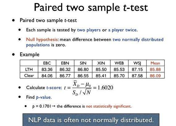
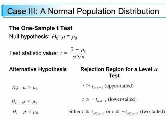
A one sample t-test is a hypothesis test for answering questions about the mean where the data are a random sample of independent observations from an underlying normal distribution N(µ, ), where is unknown.

The null hypothesis for the one sample t-test is: H 0. µ = µ 0. where µ 0 is known.

That is, the sample has been drawn from a population of given mean and unknown variance (which therefore has to be estimated from the sample).

This null hypothesis, H 0 is tested against one of the following alternative hypotheses, depending on the question posed: H 1. µ is not equal to µ
H 1. µ µ
H 1. µ µ

A two sample t-test is a hypothesis test for answering questions about the mean where the data are collected from two random samples of independent observations, each from an underlying normal distribution:

When carrying out a two sample t-test, it is usual to assume that the variances for the two populations are equal, i.e.

The null hypothesis for the two sample t-test is: H 0. µ 1 = µ 2

That is, the two samples have both been drawn from the same population. This null hypothesis is tested against one of the following alternative hypotheses, depending on the question posed. H 1. µ 1 is not equal to µ 2
H 1. µ 1 µ 2
H 1. µ 1 µ 2

Setting up and testing hypotheses is an essential part of statistical inference. In order to formulate such a test, usually some theory has been put forward, either because it is believed to be true or because it is to be used as a basis for argument, but has not been proved, for example, claiming that a new drug is better than the current drug for treatment of the same symptoms.

In each problem considered, the question of interest is simplified into two competing claims / hypotheses between which we have a choice; the null hypothesis, denoted H 0. against the alternative hypothesis, denoted H 1. These two competing claims / hypotheses are not however treated on an equal basis: special consideration is given to the null hypothesis.

We have two common situations:

1. The experiment has been carried out in an attempt to disprove or reject a particular hypothesis, the null hypothesis, thus we give that one priority so it cannot be rejected unless the evidence against it is sufficiently strong. For example, H 0. there is no difference in taste between coke and diet coke against H 1. there is a difference.
2. If one of the two hypotheses is ‘simpler’ we give it priority so that a more ‘complicated’ theory is not adopted unless there is sufficient evidence against the simpler one. For example, it is ‘simpler’ to claim that there is no difference in flavour between coke and diet coke than it is to say that there is a difference.

The hypotheses are often statements about population parameters like expected value and variance; for example H 0 might be that the expected value of the height of ten year old boys in the Scottish population is not different from that of ten year old girls. A hypothesis might also be a statement about the distributional form of a characteristic of interest, for example that the height of ten year old boys is normally distributed within the Scottish population.

The outcome of a hypothesis test test is “Reject H 0 in favour of H 1 ” or “Do not reject H 0 “.

The null hypothesis, H 0. represents a theory that has been put forward, either because it is believed to be true or because it is to be used as a basis for argument, but has not been proved. For example, in a clinical trial of a new drug, the null hypothesis might be that the new drug is no better, on average, than the current drug. We would write H 0. there is no difference between the two drugs on average.

We give special consideration to the null hypothesis. This is due to the fact that the null hypothesis relates to the statement being tested, whereas the alternative hypothesis relates to the statement to be accepted if / when the null is rejected.

The final conclusion once the test has been carried out is always given in terms of the null hypothesis. We either “Reject H 0 in favour of H 1 ” or “Do not reject H 0 “; we never conclude “Reject H 1 “, or even “Accept H 1 “.

If we conclude “Do not reject H 0 “, this does not necessarily mean that the null hypothesis is true, it only suggests that there is not sufficient evidence against H 0 in favour of H 1. Rejecting the null hypothesis then, suggests that the alternative hypothesis may be true.

The alternative hypothesis, H 1. is a statement of what a statistical hypothesis test is set up to establish. For example, in a clinical trial of a new drug, the alternative hypothesis might be that the new drug has a different effect, on average, compared to that of the current drug. We would write H 1. the two drugs have different effects, on average. The alternative hypothesis might also be that the new drug is better, on average, than the current drug. In this case we would write H 1. the new drug is better than the current drug, on average.

The final conclusion once the test has been carried out is always given in terms of the null hypothesis. We either “Reject H 0 in favour of H 1 ” or “Do not reject H 0 “. We never conclude “Reject H 1 “, or even “Accept H 1 “.

If we conclude “Do not reject H 0 “, this does not necessarily mean that the null hypothesis is true, it only suggests that there is not sufficient evidence against H 0 in favour of H 1. Rejecting the null hypothesis then, suggests that the alternative hypothesis may be true.

A simple hypothesis is a hypothesis which specifies the population distribution completely.

Examples
1. H 0. X

Bi(100,1/2), i.e. p is specified
2. H 0. X

N(5,20), i.e. µ and are specified

A composite hypothesis is a hypothesis which does not specify the population distribution completely.

Bi(100,p) and H 1. p 0.5
2. X

N(0, ) and H 1. unspecified

In a hypothesis test, a type I error occurs when the null hypothesis is rejected when it is in fact true; that is, H 0 is wrongly rejected.

For example, in a clinical trial of a new drug, the null hypothesis might be that the new drug is no better, on average, than the current drug; i.e. H 0. there is no difference between the two drugs on average. A type I error would occur if we concluded that the two drugs produced different effects when in fact there was no difference between them.

The following table gives a summary of possible results of any hypothesis test:

A type I error is often considered to be more serious, and therefore more important to avoid, than a type II error. The hypothesis test procedure is therefore adjusted so that there is a guaranteed ‘low’ probability of rejecting the null hypothesis wrongly; this probability is never 0. This probability of a type I error can be precisely computed as P(type I error) = significance level =

The exact probability of a type II error is generally unknown.

If we do not reject the null hypothesis, it may still be false (a type II error) as the sample may not be big enough to identify the falseness of the null hypothesis (especially if the truth is very close to hypothesis).

For any given set of data, type I and type II errors are inversely related; the smaller the risk of one, the higher the risk of the other.

A type I error can also be referred to as an error of the first kind.

In a hypothesis test, a type II error occurs when the null hypothesis H 0. is not rejected when it is in fact false. For example, in a clinical trial of a new drug, the null hypothesis might be that the new drug is no better, on average, than the current drug; i.e. H 0. there is no difference between the two drugs on average. A type II error would occur if it was concluded that the two drugs produced the same effect, i.e. there is no difference between the two drugs on average, when in fact they produced different ones.

A type II error is frequently due to sample sizes being too small.

The probability of a type II error is generally unknown, but is symbolised by and written P(type II error) =

A type II error can also be referred to as an error of the second kind.

A test statistic is a quantity calculated from our sample of data. Its value is used to decide whether or not the null hypothesis should be rejected in our hypothesis test.

The choice of a test statistic will depend on the assumed probability model and the hypotheses under question.

The critical value(s) for a hypothesis test is a threshold to which the value of the test statistic in a sample is compared to determine whether or not the null hypothesis is rejected.

The critical value for any hypothesis test depends on the significance level at which the test is carried out, and whether the test is one-sided or two-sided.

The critical region CR, or rejection region RR, is a set of values of the test statistic for which the null hypothesis is rejected in a hypothesis test. That is, the sample space for the test statistic is partitioned into two regions; one region (the critical region) will lead us to reject the null hypothesis H 0. the other will not. So, if the observed value of the test statistic is a member of the critical region, we conclude “Reject H 0 “; if it is not a member of the critical region then we conclude “Do not reject H 0 “.

The significance level of a statistical hypothesis test is a fixed probability of wrongly rejecting the null hypothesis H 0. if it is in fact true.

It is the probability of a type I error and is set by the investigator in relation to the consequences of such an error. That is, we want to make the significance level as small as possible in order to protect the null hypothesis and to prevent, as far as possible, the investigator from inadvertently making false claims.

The significance level is usually denoted by Significance Level = P(type I error) =

Usually, the significance level is chosen to be 0.05 (or equivalently, 5%).

The probability value (p-value) of a statistical hypothesis test is the probability of getting a value of the test statistic as extreme as or more extreme than that observed by chance alone, if the null hypothesis H 0. is true.

It is the probability of wrongly rejecting the null hypothesis if it is in fact true.

It is equal to the significance level of the test for which we would only just reject the null hypothesis. The p-value is compared with the actual significance level of our test and, if it is smaller, the result is significant. That is, if the null hypothesis were to be rejected at the 5% signficance level, this would be reported as “p 0.05”.

Small p-values suggest that the null hypothesis is unlikely to be true. The smaller it is, the more convincing is the rejection of the null hypothesis. It indicates the strength of evidence for say, rejecting the null hypothesis H 0. rather than simply concluding “Reject H 0 ‘ or “Do not reject H 0 “.

The power of a statistical hypothesis test measures the test’s ability to reject the null hypothesis when it is actually false – that is, to make a correct decision.

In other words, the power of a hypothesis test is the probability of not committing a type II error. It is calculated by subtracting the probability of a type II error from 1, usually expressed as: Power = 1 – P(type II error) =

The maximum power a test can have is 1, the minimum is 0. Ideally we want a test to have high power, close to 1.

A one-sided test is a statistical hypothesis test in which the values for which we can reject the null hypothesis, H 0 are located entirely in one tail of the probability distribution.

In other words, the critical region for a one-sided test is the set of values less than the critical value of the test, or the set of values greater than the critical value of the test.

A one-sided test is also referred to as a one-tailed test of significance.

The choice between a one-sided and a two-sided test is determined by the purpose of the investigation or prior reasons for using a one-sided test.

Example Suppose we wanted to test a manufacturers claim that there are, on average, 50 matches in a box. We could set up the following hypotheses H 0. µ = 50, against H 1. µ 50 or H 1. µ 50 Either of these two alternative hypotheses would lead to a one-sided test. Presumably, we would want to test the null hypothesis against the first alternative hypothesis since it would be useful to know if there is likely to be less than 50 matches, on average, in a box (no one would complain if they get the correct number of matches in a box or more). Yet another alternative hypothesis could be tested against the same null, leading this time to a two-sided test: H 0. µ = 50, against H 1. µ not equal to 50 Here, nothing specific can be said about the average number of matches in a box; only that, if we could reject the null hypothesis in our test, we would know that the average number of matches in a box is likely to be less than or greater than 50.

A two-sided test is a statistical hypothesis test in which the values for which we can reject the null hypothesis, H 0 are located in both tails of the probability distribution.

In other words, the critical region for a two-sided test is the set of values less than a first critical value of the test and the set of values greater than a second critical value of the test.

A two-sided test is also referred to as a two-tailed test of significance.

The choice between a one-sided test and a two-sided test is determined by the purpose of the investigation or prior reasons for using a one-sided test.

Example Suppose we wanted to test a manufacturers claim that there are, on average, 50 matches in a box. We could set up the following hypotheses H 0. µ = 50, against H 1. µ 50 or H 1. µ 50 Either of these two alternative hypotheses would lead to a one-sided test. Presumably, we would want to test the null hypothesis against the first alternative hypothesis since it would be useful to know if there is likely to be less than 50 matches, on average, in a box (no one would complain if they get the correct number of matches in a box or more). Yet another alternative hypothesis could be tested against the same null, leading this time to a two-sided test: H 0. µ = 50, against H 1. µ not equal to 50 Here, nothing specific can be said about the average number of matches in a box; only that, if we could reject the null hypothesis in our test, we would know that the average number of matches in a box is likely to be less than or greater than 50.

A one sample t-test is a hypothesis test for answering questions about the mean where the data are a random sample of independent observations from an underlying normal distribution N(µ, ), where is unknown.

The null hypothesis for the one sample t-test is: H 0. µ = µ 0. where µ 0 is known.

That is, the sample has been drawn from a population of given mean and unknown variance (which therefore has to be estimated from the sample).

This null hypothesis, H 0 is tested against one of the following alternative hypotheses, depending on the question posed: H 1. µ is not equal to µ
H 1. µ µ
H 1. µ µ

A two sample t-test is a hypothesis test for answering questions about the mean where the data are collected from two random samples of independent observations, each from an underlying normal distribution:

When carrying out a two sample t-test, it is usual to assume that the variances for the two populations are equal, i.e.

The null hypothesis for the two sample t-test is: H 0. µ 1 = µ 2

That is, the two samples have both been drawn from the same population. This null hypothesis is tested against one of the following alternative hypotheses, depending on the question posed. H 1. µ 1 is not equal to µ 2
H 1. µ 1 µ 2
H 1. µ 1 µ 2